Robotics Exploration
Published:
I had the opportunity to work with some of the UVA Collaborative Robotics lab’s robots throughout my second semester. I followed several research directions, as I learned about various components of robotic learning.
Early Imitation Learning
Date: Late December
Joint Velocity Prediction
Problem Formulation. Given a set of demonstrations for a task, can we learn to perform that task? We formulate this problem as “next keypoint prediction", in which given a state \(s\), we aim to predict the action \(a\) (that is, an \(SE(3)\) end-effector position and rotation) that accurately imitates the demonstrations towards completing the task.
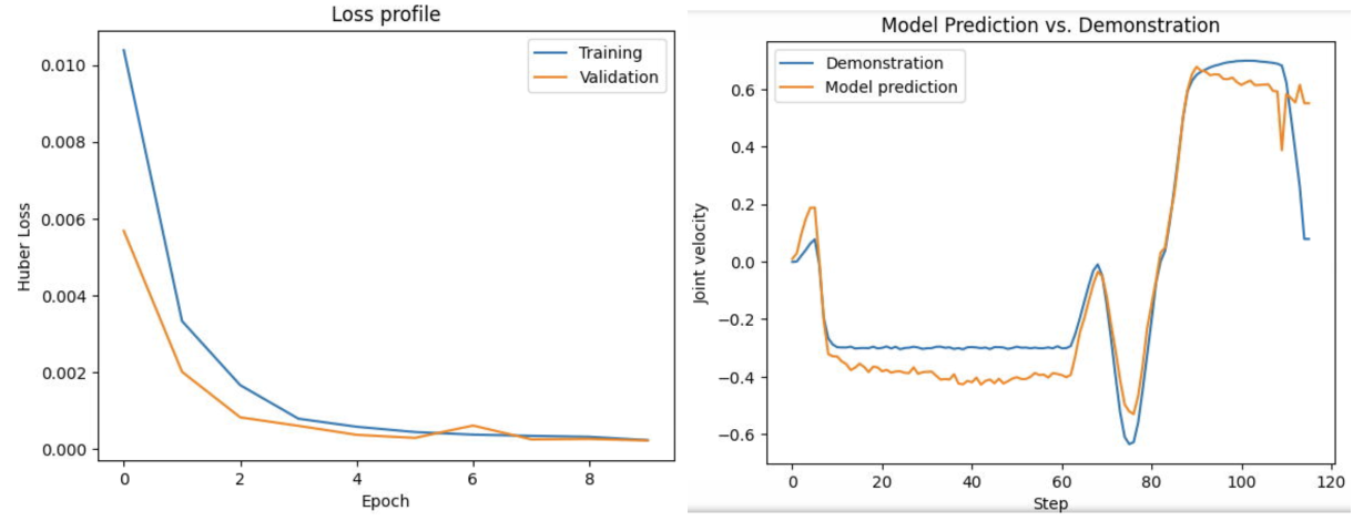
Experimental Setup. I used CoppeliaSim and a small set of tasks from the RLBench repository [@rlbench]. Because it was time-consuming to generate new demonstrations online, I used a set of prepopulated task demonstrations from the PerAct repository [@peract]. The training objective was Huber loss (a type of mean-squared error meant to be robust to outliers) trained on joint velocities (\(\dot q\)): \(\mathcal{L}_{huber} = \begin{cases} \frac{1}{2}(\dot q - \hat {\dot q})^2 & \text{if } |\dot q - \hat {\dot q}| \leq \delta \\ |\dot q - \hat {\dot q}| & \text{if } |\dot q - \hat {\dot q}| > \delta \end{cases}\) I experimented with two image encoders: the vision transformer backbone from CLIP [@clip], and ResNet18 [@resnet] (pretrained on ImageNet). One thing I did not realize at the time, but think would have been interesting to compare, would be to use the vision transformer backbone for CLIP and to compare it to the ResNet backbone for CLIP. I believe this would have elucidated, in a more controlled manner, whether convolutional neural networks or vision transformers have the advantage in robotic manipulation. My intuition at this point tells me that vision transformers are better for “where" inferences, and that convolutional models are better for “what" inferences.
Results. I found that CLIP is a strong feature extractor compared to the ResNet. In particular, it was able to predict joint velocities with relatively high efficacy. I now realize that this is potentially because of the ability for the CLIP vision transformer to utilize positional embeddings, whereas ResNet models are translation-invariant. As an inductive bias in object detection, this is great, but when action outcomes can be dependent on position within an image, position-sensitive models may be better.
Keypoint-Conditioned Imitation Learning
The next iteration on this was to do keypoint-conditioned imitation learning, rather than directly predicting joint velocities. The hypothesized advantage is that keypoints are simpler to predict, which should make learning easier.
Experimental Setup. Here, I adopt a scheme similar to RVT [@rvt] (Robotic View Transformer) and PerAct [@peract] (Perceiver-Actor). Given a set of demonstrations – particularly, a set of observations (RGB images) and robot states (end-effector positions and rotations) – I extract keyframes, and then create a small dataset in which observations are mapped to the “next keyframe".
Keyframe Extraction is done with a simple heuristic: Whether the gripper state changes, or whether there is a change in velocity. Keyframe extraction is simple for demonstrations that occur in simulation, because motion is piecewise linear. It is also possible to extract keyframes from human demonstrations [@waypointslxs].
Simple Experiment: Vision Transformer Token Head. Aforementioned RGB observations (images multiple input directions) have future keypoint locations (members of \(SE(3)\)) projected onto them according to camera matrices. I used a pretrained vision transformer (CLIP) trained with cross-entropy loss to identify future keypoint locations.
Aside: Vision Transformers: Vision transformers [@vit] (ViTs) tokenize images by (1) (optional preprocessing step, not used everywhere) resizing them to \(224 \times 224\) and potentially scaling pixel values, and (2) breaking up the preprocessed image into tokens (often, these are \(14 \times 14\) or \(16 \times 16\) chunks of pixels). These raw tokens (which can be thought of as the word embeddings before a language-based transformer) are encoded through the transformer layers, resulting in contextualized features. For my approach, I simply take an overhead input image and train a classification head for whether a certain token contains the future keypoint.
Aside (Camera Projection Matrices): Given a Cartesian keypoint location \($[\vec x] = [x, y, z, 1]^\top\)$ in robot frame (with homogeneous coordinates), then for each camera, there exists a camera matrix \(M \in \mathbb{R}^{3 \times 4}\) such that \([\vec y] = M [\vec x] \in \mathbb{RP}^2\) is a pixel location. Basically, multiply by the matrix, and turn robot coordinates into pixel locations. This matrix, if you are trying to self-teach, is finicky to construct.
Simple Experiment: Voxelization. Following the Robotic View Transformer from Nvidia, I took point clouds and applied a voxelization step followed by a rendering step. I created my own voxelizer to do this because I was having problems with pytorch3d. I rendered “virtual views" along the orthogonal coordinate axes, and applied the aforementioned keypoint prediction pipeline. This resulted in decent-ish results. However, I was never able to quantify them strongly, nor test them in closed loop.
Aside: Voxelization: To perform voxelization, I defined workspace boundaries (\(\vec x_{min}\) and \(\vec x_{max}\) in robot coordinate system) and discretized the coordinates into buckets. Each 3-tuple of coordinates formed a voxel, which was assigned an occupancy level (\(\alpha\)) and a color (\(c\)). Then, I created a voxel renderer along each axis, through a rendering technique very similar to NeRF: creating rays parallel to the view axis (using an orthographic projection, so all such rays were parallel), and marching them forward. As an example, if the workspace along the \(z\) axis ranges from \(z_{near}\) to \(z_{far}\), I calculate the final pixel value in the image as \(\hat c(x, y) \gets \alpha_n c(x, y, z_n) + (1 - \alpha_n) \hat c(x, y)\) iterating from \(z_n = z_{far}\) to \(z_n = z_{near}\), with \(\hat c(x, y)\) representing the final pixel value for the \(z\) axis image. \(\hat c(x, y)\) is initialized as \((0, 0, 0)\) to give images a black background.
TAKEAWAY: Try things in closed-loop. Keep going until they work!
In-Context Learning
Date: Early January
One motif that I was interested in (since the beginning of the lab) was in-context learning. My vision was to create a robot for which you could explain tasks in natural language, and have the robot ultimately perform them for you. However, I think I did not realize how challenging this would be, because I did not stop to think about what pieces would be necessary.
Background Reading. There was an object-centric prompting mechanism [@vima] and meta-learning [@adaptiveagents] set of papers which were cool cool. I do not believe that I understood them deeply. I also designed an approach to use a temporal (i.e., multiple input-image) vision transformer to predict future actions conditioned on previous actions. Finally, I considered that it was important to train policies to run on the actual robot. I made a couple of setups:
Pick Same Object. Sequences of two images. The first would have a certain item circled. The second would have the items shuffled, and the target label would be the item that was circled.
Squares. I made a prompt:
observe the <color> square, and continue the pattern.Left, Right, Red, Blue. A flag would be set in the model input, prompting it to change its selection behavior between left/right side of an image, or red/blue side of an image.
It took a surprising amount of compute for the model to learn which one to use with in-context instructions. It was easy to train the model to make predictions for single tasks, though. Some of the things I learned were:
Learning rate is important in transformers. Dynamic learning rate schedules can be important as well. For example, without a linear warmup, some transformer models will simply never converge, or it would take forever to work. After the linear warmup, some form of annealing is good.
Without pretraining, in-context learning is fairly difficult.
Using a Real-Life Robot
Date: Early February
AprilTags
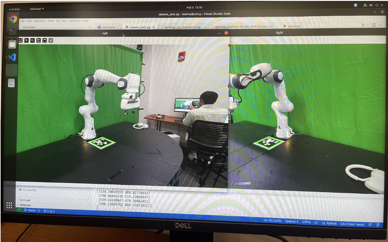
I wanted to try working on a real-life robot. I started by working with a pair of Azure Kinect RGBD cameras, and an AprilTag. To interact with cameras, I use the pyk4a library on GitHub, which requires the proprietary libk4a package (which is unfortunately only available in binary form). I used the apriltag library on GitHub, which provides the pixel locations of each AprilTag’s corners. Using the built-in camera intrinsic parameters, distortion coefficients, and known coordinates of the AprilTag in robot frame, it is possible to calculate a perspective-and-point (PnP) transform, which essentially determines the extrinsic matrix of the camera. Note that this is susceptible to noisy measurements of AprilTag coordinates, or inaccurate AprilTag placement. I (much later) go on to develop a more sophisticated and robust calibration system, which results in strong results after just 1-2 minutes of calibration per camera. The ability to place point clouds in robot frame allows for point clouds from different perspectives to be fused.
Using Offline Data
I tried to use some existing data we had collected. Some notes for future work:
Ensure timestamps are correct: In addition to being unsynchronized, I ran into the surprising issue that dependent on the run, images and robot control commands were collected with trial-dependent time offsets. This made it a bit difficult to do anything with the offline data.
Use a standardized setup: It was also difficult to create correct mappings from robot state space to pixel space.
At this point I tried to label 3D keypoints visually. That is, given two camera views, I specified target locations by manually selecting the target location as 2D coordinates. As a result of my camera calibration, I was able to have a robot move to a precise 3D location, simply using 2D information. This was an important moment because I realized that 2D image information could be highly useful for robotic policies.
Video Diffusion Models
Date: Late February to Early March
I then decided that large pretrained diffusion models would be good for robotic manipulation. I recognized that many problems in robotic control, similar to large language models with transformers, can be reduced to the form “generate a video of a robot performing X action", conditioned on the robot’s previous observations. There were several signals that would indicate positive performance in this direction. (1) Diffusion Policy [@diffusionpolicy] was demonstrating impressive multimodal (“multi-solution") planning capabilities in robot state space. (2) Image inpainting and video prediction models seemed to be doing well as well [@videolanguageplanning; @susie]. (3) Sergey Levine and Chelsea Finn created a patent for image prediction-based methods for robotic planning (although I think other works had done it earlier?). This may appear true, at least superficially.
I made a presentation of some existing video diffusion methods (view here). Still think I should have thought more logically / at a higher level about this one though, even if the theory was technically there. It’s important to consider the compute and talent budgets that other labs have to execute on more ambitious ideas.
Regardless, I decided to just try this out. I learned how to train large models on multiple A100 GPUs, but I think I could have saved a lot of time lol by focusing on more direct parts of the project and saving this for future work. I learned about EDM preconditioning strategies for diffusion models [@edm], which essentially dictate the loss function weighting at each training diffusion timestep, and the tradeoff between predicting \(x_0\) and predicting \(\epsilon\). I also rederived the forward diffusion reparameterization trick.
For training, I used a pretrained Stable Video Diffusion (SVD) [@stablevideodiffusion] model, and modified an existing HuggingFace training script for the image-based Stable Diffusion. This was harder than I anticipated, because the model architectures were different, and it was my first time training a diffusion model in such a way. In fact, this was so difficult that in order to check my sanity, I followed a guide from nn.labml.ai and trained/implemented my own diffusion model on MNIST. Yang Song and Lilian Weng’s blogposts is a great place to learn how diffusion models work.
In terms of learning about diffusion, I learned about the importance of the signal-to-noise ratio schedule: It should go from \(1\) to \(0\) [@fixtheschedule], this is much easier to tune correctly than a \(\beta\) schedule; besides, you can derive a \(\beta\) schedule from a signal-to-noise ratio, and I think the signal-to-noise ratio is more interpretable. Offset noise is also important to be able to sample very bright or very dark images from diffusion models. I also learned about the importance of the sampling step. You can get significantly better results with slightly under-optimized diffusion models simply by applying more backward inference steps. From a standpoint of annealed Langevin Dynamics, this allows the model to make more corrections at a given noise level, which seems to stabilize things. This all sort of ties into a great underlying theme about the success of diffusion models: They allow ML models to specify cost functions / local gradients (the score function), which are significantly easier to learn than direct samples from the probability distribution. The point is, it is easier to detect mistakes than to generate a satisfying sample directly.
This whole principle that diffusion models are optimizers allows for striking out-of-the-box capabilities. One example is that of optical illusions created by diffusion models [@diffusionillusions].
Anyway. I’m getting sidetracked. Here’s more training details about the video diffusion model. I trained my models on the RT-1 dataset from Google [@rt1]. I formatted the dataset by taking \(25\)-frame chunks (which is what SVD was finetuned for), using no text conditioning (I just wanted to get video diffusion working whatsoever). The results are conditioned on the initial image, the features of which are concatenated to the noisy latents of all future frames to guide generation. I used the HuggingFace Accelerate library, which includes advanced techniques for distributing workloads to multiple GPUs, for training. Overall, I used 10k samples and trained for 2 epochs. The result was a model capable of generating relatively decent results for the compute budget I had. I initially experimented with LoRA to save memory, but I found that the model did not improve enough if I did that.
One important detail that I had not noticed before during training was the impact of the VAE. Misconfiguring the VAE = death for your training. I did not realize that the VAE was trained with a scaling parameter, and during my finetuning, I at one point was training without regard for that. And thus, I deviated too far from the pretraining distribution, resulting in subpar performance for a bit. Once this was fixed, video generations looked significantly better.
Diffused Image from My Model
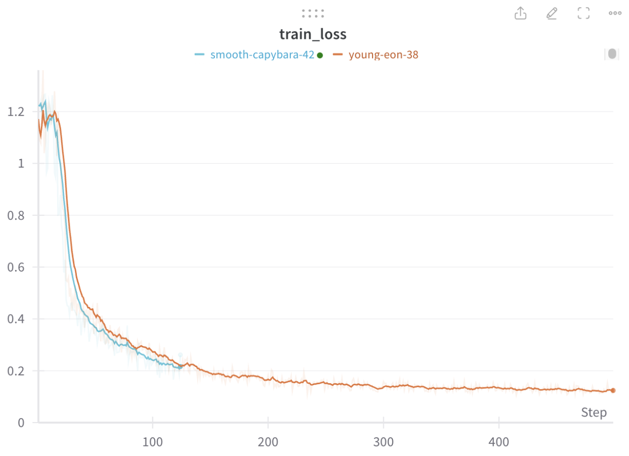
Loss Curve for Diffusion Training
Considering the lower-level details in retrospect, there are many reasons this should not have worked:
Compute limitations. Pretrained diffusion models require massive amounts of compute, and I was not a researcher on model efficiency, I was a researcher in robotics. Additionally, it is unclear whether video diffusion models even should be the standard for motion planning and prediction. Sure, it makes sense to make prediction in image space in some sense, but there are also many more practical approaches that should work equally well before getting to a point where that would make a difference.
Implementation limitations. Even with a trained diffusion model, performing evaluations on such a model would be difficult, when considering how it would look in material form. This would require some form of visual servoing, or otherwise, some model to encode the action space (serving as the dynamics model as a function of actions), and some model to extract meaningful reward information about future states (a reward model).
2D Diffusion Models
Date: March
Note: I found that concurrent work actually implemented what I was thinking about doing here. This paper is called Render and Diffuse, and it came from the Dyson Robot Learning Lab. [@renderanddiffuse].
One valid question I had, after seeing that much robotic planning could be performed in 2D space, was to use diffusion over images. This is already sort of what Diffusion Policy does (in retrospect). There were many theoretical reasons for this though:
Access to internet-scale pretraining. There are a ton of image-language pretrained transformers that are capable of a wide range of downstream tasks. Additionally, such transformers demonstrate great scene understanding.
Compute efficiency. Video diffusion models are extremely costly. Performing diffusion in action space instead is much better.
Analogies to visual servoing. Humans primarily measure motor errors visually. Therefore, it should seem natural for an agent to be able to correct its movements given an input image and proprioception, and in the best case, this reduces to a deep-learned version of visual servoing.
There are some issues though with this approach:
Simpler prior work: At a high level, this approach purports to have exactly the same benefits as the well-established Diffusion Policy [@diffusionpolicy]. Therefore, I should have worked with that.
Insufficiency of 2D corrective terms: My model outputted 2D correction terms, and my hope was that by optimizing the score function across all views simultaneously, I would eventually reach a mode of the joint probability distribution \(\pi(x, y, z | o)\). However, this is simply not true. A maximizer of \(P(x, y)\), \(P(y, z)\), \(P(z, x)\) is not necessarily a maximizer of \(P(x, y, z)\); there is too much ambiguity.
I created a noise-conditioned score matching model, where conditional on the noise level, each output token of a vision transformer would include a direction to move to the nearest mode. The training loss was as follows. For a token at position \((x, y)\), and true keypoint position at \((x_0, y_0)\), predicting the noise \(\hat \epsilon\) and quaternion map \(\hat q\), the loss function was as follows: \(\mathcal{L} = \underbrace{\frac{1}{\sigma^2}((x - x_0) - \hat \epsilon)^2}_{\text{translation noise}} + \underbrace{(\hat q - q_0)^2(e^{-(x - x_0)^2/\sigma^2})}_{\text{quaternion field}}\) Where \(\sigma\) is the standard deviation used by noise conditioning. The quaternion loss was used to enable prediction of end-effector rotations at multiple modes; broadly encouraging nearby quaternion predictions to be the same, but not penalizing distant quaternion predictions for one mode when they were correct for a closer mode. The result was a model that seemed capable of predicting keypoints. Below I have some images:
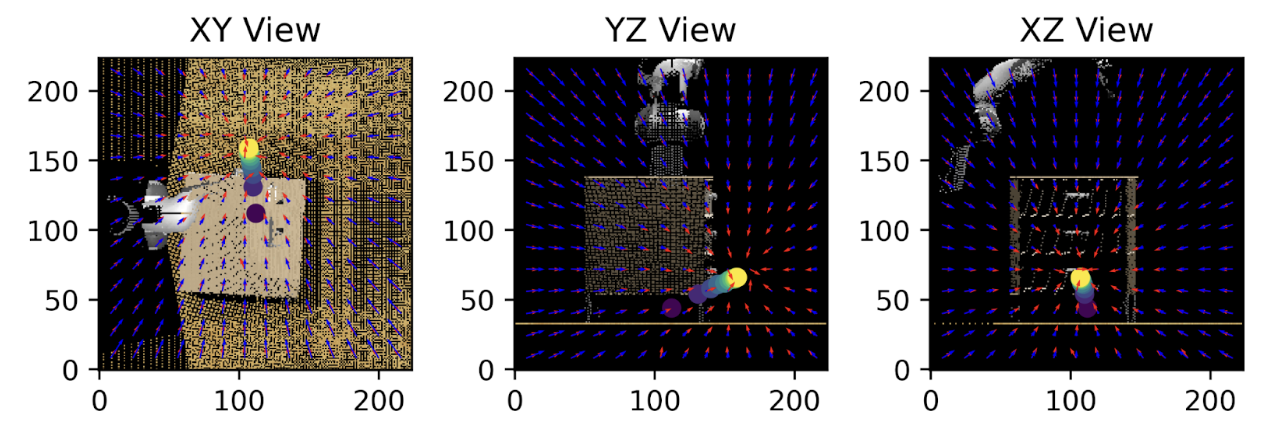
2D Keypoint Diffusion
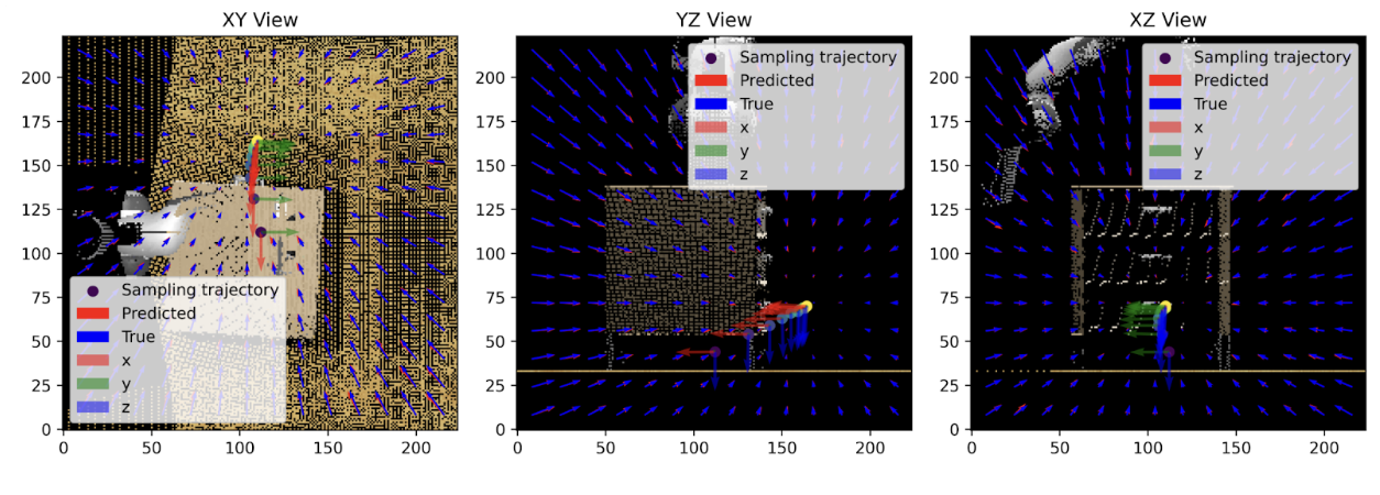
Rotation Angle Prediction
I was actually able to get virtual plan rendering working, which was deceptively difficult! This required loading the URDF files and a 3D model into a 3D rendering environment, and using the quaternions and translation vectors to calculate where the end-effector should land in the scene. I don’t think I ever ended up doing anything with this though.
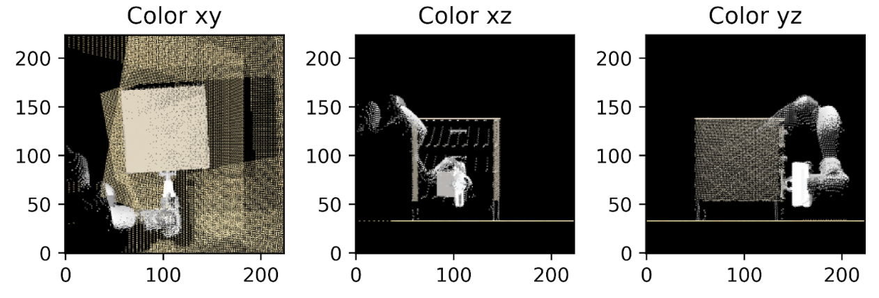
Virtual Plan Rendering
Language Models for Planning
After I realized that it was mathematically impossible for my formulation of 2D diffusion to work (optimizing from multiple views), I decided to pivot towards using language models as planners. The primary reason for this is their impressive zero-shot capability: Language models are great for code generation, and have an impressive prior over general world knowledge. With a bit of fine-tuning, they should perform excellently for robotic control tasks. One line of work on language models for robotic planning, particularly for long-horizon robotic planning, envisions the use of a language model that processes observations about the environment via external APIs called via tool use [@innermonologue] or code generation [@codeaspolicies; @voxposer; @progprompt].
There are also some interesting open questions for language models:
Closed-loop control: Language models generate code policies for multiple timesteps. Executing these code policies without checking for task execution errors isn’t a great idea. What ways are there to use VLMs as “error checkers"?
Instruction memory: Can we encode instructions and use language models to “recall" desired behavior in the future? What ways are there to implicitly create this type of memory?
Visual grounding: When (vision) language models reason, it is hard to connect their reasoning to the images they refer to. However, if we could reason over grounded objects, we could unlock significantly more advanced planning capabilities. This is still an open question and something I am interested in exploring further.
I explored the first and third points by creating an agentic LLM planner. Particularly, I created a notion of an “event stream", in which observations, actions, rationales, and reflections would enter a shared space for future reference by the language model.
There was also a ton of engineering effort required to make this into a reality. First, there was camera calibration to be able to fuse RGBD point clouds in robot space. Then, there was camera-robot calibration, which adjusted the resulting detections. Finally, there was grasp synthesis, and execution on the robot control system.

Object Detection and Selection
Plan generation. Based on previous actions taken, the current instruction, and the current image observation, the VLM generates a plan for how to interact with the objects in scene.
Code generation. Based on the reasoning generated by the VLM, I then use a separate prompt to generate code to control the robot. I expose a small set of APIs:
Object detection: This returns objects with 3D point clouds in robot frame, conditioned on a target text label.
Relative motion: This allows the robot to translate or rotate its end-effector by a calculated amount, in meters. This is useful, for example, for lifting items up simply by performing an upward translation.
Absolute motion: This allows motion with respect to anchor coordinate locations. One example for why this might be useful is if the robot arm needs to move above a certain item to pick it up.
Gripper control: This allows the robot to open or close its gripper. Additional logic adjusts the grasp axis to perform a force closure, through a rough (and non-robust) heuristic I made.
Object selection. I used an OwlV2 [@owlv2] model (which is great for open-vocabulary object detection) to locate objects of a specific type. To choose specific objects based on fine-grained attributes (like color, text, etc.), I create image crops centered around each of the object detections, and ask the VLM to describe the physical attributes of those objects. Then, these descriptions are compiled into a summary (a list of lines Object 1: <Description>\nObject 2: <Description>\n ...), before the VLM makes its final decision for which object to select, or none of the objects if none match.
Object point cloud extraction. Once an object has been located in a 2D image, we must further ground it in a 3D location. This is done in two steps. The first step is to use the Segment Anything Model [@sam] to generate an image segmentation. Because images are in RGBD, this image segmentation automatically generates a set of object points in robot state space. However, these object points only represent one side of the object, and grasp planning with this will not work. To fix this, I use a camera on the other side of the robot, as depicted below.
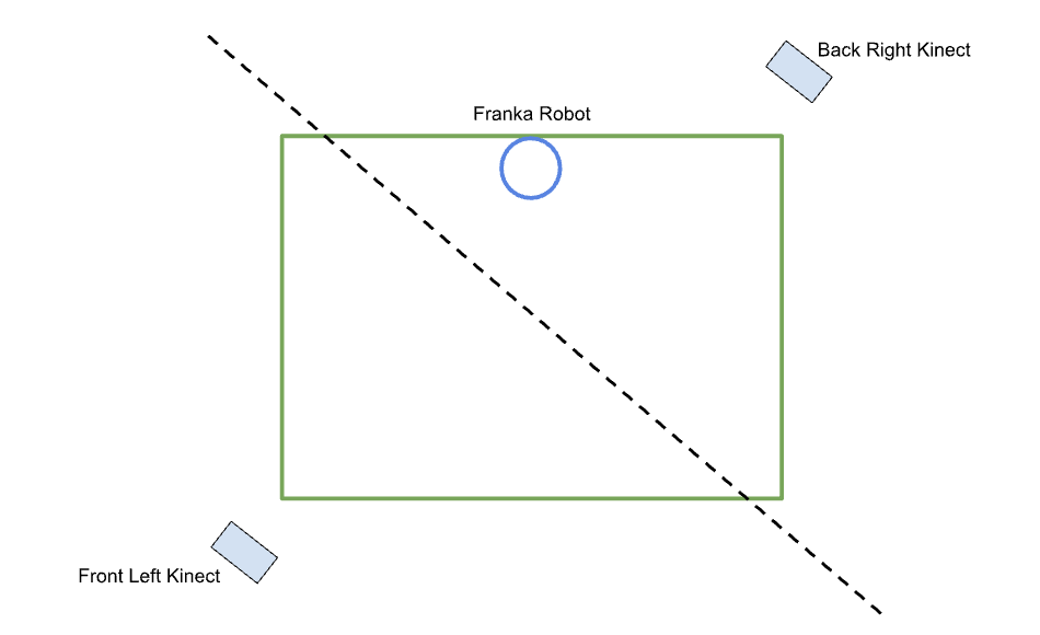
Camera Layout
Camera-Robot Cross Calibration. To create accurate calibrations of images to robot state, I wrote a script that (1) allowed a user to place a block with an AprilTag on it in the robot’s gripper, and (2) moved the AprilTag block to predefined locations in a 3D cubic grid. I then logged robot state information directly from the robot (rather than using the waypoint as a ground truth) due to control error. Using the correspondences between image pixel locations from the center of the AprilTag, and the known positions in robot coordinate space, I was able to use OpenCV’s solvePnP function to create a more accurate camera extrinsic calibration than the original AprilTag approach described earlier.
Robot Control. Robotic control was done with Polymetis, a framework that allows specialized control policies to be deployed at a high frequency. It includes a barebones min-jerk motion planner as well. Control is done with PID over joint positions/velocities in a tight loop rather than model predictive control. I found that this mostly worked out of the box except for two major challenges:
Flange frame miscalibration: For some reason, all actions the robot took were offset by \(10.34\) centimeters downward, and with a rotation of \(\pi/4\) radians around the z axis. Other people experienced this too (here).
Improper control coefficients: This was much easier to discover and debug. I found that the robot sagged under gravity at times, and was otherwise susceptible to slight pushes; to fix this, I increased the proportional gain in the PID.
I also used a very simple motion planning heuristic to reduce the number of collisions with items on the table. First, whenever the robot’s Z value was anticipated to move downward during a motion, I would first make the horizontal motion, and then the downward motion. If a movement involved upward motion, I would make the upward motion first, and then the horizontal motion. The overall result from this is that most of the horizontal motion occurs at higher Z levels, resulting in fewer collisions for basic tabletop tasks.
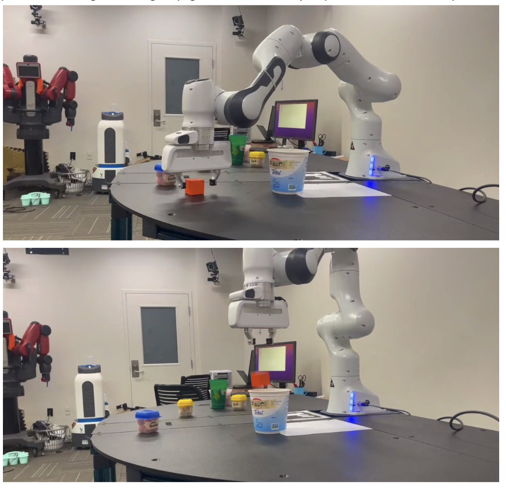
Robot Completing a Task
Grasp Generation Heuristic. When the robot attempts to grasp a target object, it uses a grasp generation heuristic I created. This voxelizes the object point cloud, rotates the voxels on their side, and rotates around the (former) z-axis, looking for appropriate planes to grasp along. This plane estimation approach is highly non-robust, and simply uses the slope of the voxelization at the top and bottom of the object to calculate the angles (\(\alpha\)) that dictate the amount of friction generated. Hole-filling or other techniques would make it better. A score is calculated based on these angles of approach which determines whether there is enough friction to perform the grasp. This is based on the Fast Force Closure algorithm by Van-Duc Nguyen [@fastforceclosure]. I found that this approach was capable of correcting gripper rotation angles for objects rotated at 45 degrees, enabling more successful grasps.
Object Memory for Language Models
I performed some additional experiments to create a sort of “visual object memory" for language models. For example, when looking at a snickers bar, a robot should be able to recognize that it contains peanuts, and thus not recommend it to someone with a peanut allergy. In retrospect, this set of experiments was hard to test, and it was not clear there was high demand for this sort of feature compared to other, high-priority components. To implement a non-verbal form of object memory, I used the following technique:
CLIP heatmap of the scene: I used the MaskCLIP reparameterization trick [@maskclip] to create text-aligned, dense CLIP features. The trick works by replacing the final transformer layer in the CLIP ViT: instead of applying self-attention, we perform a value projection on each token, and project from image embedding space to the multimodal text-image embedding space. To enable CLIP heatmaps to be created from images of arbitrary aspect ratios, I use positional encoding interpolation from the original ViT paper and DINO [@vit; @dino], which I borrow from the Distilled Feature Features [@featurefields] GitHub repository. Essentially, this reshapes the \(16 \times 16\) grid of positional encodings built into CLIP and applies a bilinear interpolation to any arbitrary grid size desired. Finally, I take the token-level CLIP features and interpolate them into pixel space.
Registration of object features: Given an object segmentation obtained via SAM, I then segment the pixel-level CLIP features to create a positive set (inside the segmentation) and negative set (outside the segmentation). I also augment these sets with Gaussian blurs, slight rotations, and background removal. Finally, I reweight the classes to 25% positive features, and 75% negative features, before applying a Support Vector Machine [@svm]. I found it to be crucial to perform class reweighting and data augmentation to increase the robustness of the classification. I used SVMs because of their ability to output well-calibrated class probabilities compared to a naïve dot product. Another reason for using SVMs is that they can use any kernel for classification, be it a linear function (as I used) or radial basis functions (which represent a mixture of Gaussians).
Object tracking: To further augment object features, I used XMem [@xmem], a method aimed at generating continual object segmentations in video. This seemed highly capable and generally worked for tracking objects as they rotated in a scene to enable fast collection of additional features.
Instance segmentation: After creating a feature detector, I needed to be able to reconstruct accurate object segmentations. Given a new RGB image of a scene, I extracted dense token-level CLIP features in the same way as before. I used a threshold to identify positive features and create a mask. Then, I encoded the input image with SAM and prompted it with randomly-selected points within the mask. Any masks that had sufficient duplication with other masks (e.g., IOU > 0.7) would be removed, and any masks which seemed to be false positives (e.g., positive features only made a small fraction of the resulting mask) were also discarded.
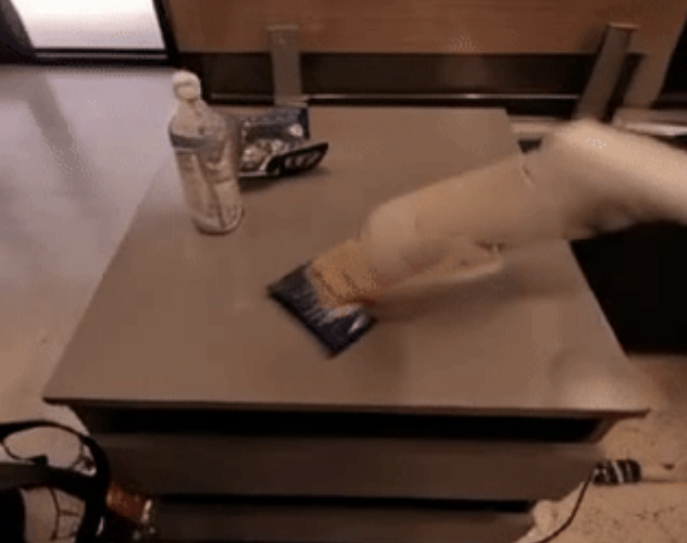
Result: Below is an image of one-shot object segmentation. In this case, the model is given a small set of annotations for a certain type of food packaging, and is able to recognize the target object regardless of distractors in the scene.
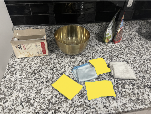
One-shot object segmentation
Alas, after this, I did not perform a closed-loop test of whether this could be used to modify a robot’s behavior.
Visual Grounding for Language Models
Date: May
I realized rather quickly for VLMs that a really important question is whether we can have VLMs output spatial locations rather than just language. That is, whether the objects of their reasoning can be grounded in the input image. One way to do this is to first generate all objects in a scene, and then detailed descriptions for each of these objects, and finally, select the optimal object out of that stack.
Can we have language models which reason about objects in a grounded manner? One compelling ideal outcome is to have the same reasoning capability as textual chain-of-thought, but for scenes. To experiment with this, I use the test task of generating referring expressions and detailed object captions given bounding boxes. Compared to other approaches, though, which might require reencoding an image crop for every object in a scene, allows one to directly decode object captions prompted by bounding boxes. In addition to improved computational speed, we can reason about objects within bounding boxes in terms of the surrounding context, which is impossible to do when just describing an object based on its cropped image.
Vision-Language Models Effectively Extract Object Attributes. I found that when using excellent vision-language models (such as GPT-4V), accuracy increases significantly for tasks requiring references to specific object attributes. For example, whereas a simple image embedding might capture the general type of an object, generating object captions with a vision-language model (which have more tokens allocated to represent larger and potentially more complex objects) allows for more granular detail, even compared to approaches that claim to “unleash extraordinary object grounding", like Set-of-Mark prompting [@setofmark]. However, in my opinion, it is unclear still whether these results are due to superior attribute extraction or due to the choice of vision model used (in our case, GPT-4V, which has who knows how many parameters, compared to OwlV2, which has a couple hundred million parameters).
| Object Category | Ours | SOM | MaskCLIP Alignment | Cropped Image CLIP Alignment |
|---|---|---|---|---|
| Cups | 75.00 | 44.44 | 55.56 | 33.33 |
| Condiments | 85.71 | 16.67 | 35.71 | 26.19 |
| Spoons | 60.00 | 12.00 | 40.00 | 34.00 |
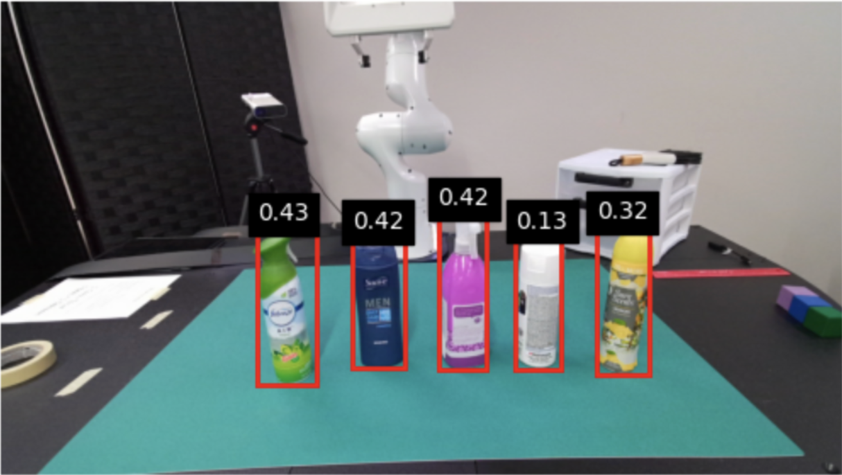
A set of visually-similar objects
Pretraining with Object Classification. I initially trained the multimodal projection layer and sequence modeling components of PaliGemma with object classification. Particularly, I prompted the model to classify an object corresponding to a bounding box (represented as four <locXXXX> tokens in xyxy format), and set the target to be the text representation of the MSCOCO class name. When applied to the train2014 split of MSCOCO, this provides approximately 600000 training examples, spanning 80000 images. This provides high object detection density per image, forcing models to respect bounding box information to generate correct labels.
Finetuning with Referring Expressions: OCID-Ref and RefCOCO. I found that OCID-Ref [@ocidref] seemed to be a good dataset for referring expression comprehension. Importantly, it had a high density of objects per image, making it a great way to train object captioning models with strong respect for spatial locations. The RefCOCO datasets [@refcoco] were also great for this. I fine-tuned PaliGemma to generate referring expressions for objects given bounding boxes. I then ran an experiment to see whether objects could be correctly disambiguated based on their referring expressions.
Finetuning with Descriptive Captions: Synthetic Data Approach. I generated a small dataset of \(5000\) object-centric captions for finetuning, using the Phi-3 Vision [@phi3] model from Microsoft to extract object attributes for a large set of object detections in the MSCOCO dataset. I found that including the class of object in the prompt was crucial to generate attributes correctly, as otherwise, models would misclassify objects and describe corresponding features incorrectly due to the lack of surrounding context. Additionally, I prompted Phi-3 to describe physical attributes of the images only, as it would otherwise hallucinate features that correspond to the target object that were not explicitly visible, or misclassify visible features. I finetuned PaliGemma on this dataset for \(4\) epochs.
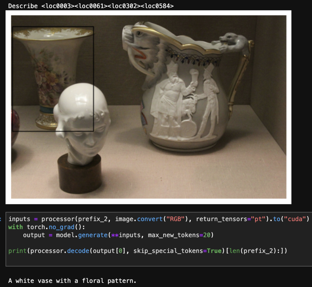
A detailed object caption
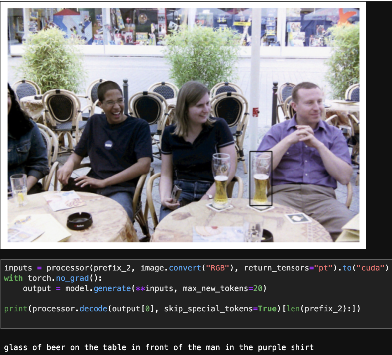
A referring expression generated from an object bounding box
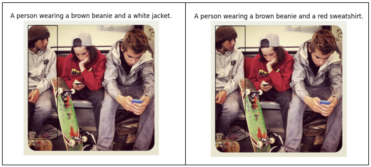
Left: No object pretraining; Right: Object pretraining
Conclusion
I learned a lot from this experience. In retrospect, much of the research that was performed here was close to being a rich project, and simply required more pointed investigation and testing.
Acknowledgements
I would like to thank Mohammad Samin Yasar for his continual support of my work, even during the week I returned to Charlottesville to try to get something working, and for teaching me how to use the robots in the lab.
References
Black, Kevin, Mitsuhiko Nakamoto, Pranav Atreya, Homer Walke, Chelsea Finn, Aviral Kumar, and Sergey Levine. 2023. “Zero-Shot Robotic Manipulation with Pretrained Image-Editing Diffusion Models.” https://arxiv.org/abs/2310.10639.
Blattmann, Andreas, Tim Dockhorn, Sumith Kulal, Daniel Mendelevitch, Maciej Kilian, Dominik Lorenz, Yam Levi, et al. 2023. “Stable Video Diffusion: Scaling Latent Video Diffusion Models to Large Datasets.” https://arxiv.org/abs/2311.15127.
Brohan, Anthony, Noah Brown, Justice Carbajal, Yevgen Chebotar, Joseph Dabis, Chelsea Finn, Keerthana Gopalakrishnan, et al. 2023. “RT-1: Robotics Transformer for Real-World Control at Scale.” https://arxiv.org/abs/2212.06817.
Burgert, Ryan, Xiang Li, Abe Leite, Kanchana Ranasinghe, and Michael S. Ryoo. 2023. “Diffusion Illusions: Hiding Images in Plain Sight.” https://arxiv.org/abs/2312.03817.
Caron, Mathilde, Hugo Touvron, Ishan Misra, Hervé Jégou, Julien Mairal, Piotr Bojanowski, and Armand Joulin. 2021. “Emerging Properties in Self-Supervised Vision Transformers.” https://arxiv.org/abs/2104.14294.
Cheng, Ho Kei, and Alexander G. Schwing. 2022. “XMem: Long-Term Video Object Segmentation with an Atkinson-Shiffrin Memory Model.” https://arxiv.org/abs/2207.07115.
Chi, Cheng, Zhenjia Xu, Siyuan Feng, Eric Cousineau, Yilun Du, Benjamin Burchfiel, Russ Tedrake, and Shuran Song. 2024. “Diffusion Policy: Visuomotor Policy Learning via Action Diffusion.” https://arxiv.org/abs/2303.04137.
Dong, Xiaoyi, Jianmin Bao, Yinglin Zheng, Ting Zhang, Dongdong Chen, Hao Yang, Ming Zeng, et al. 2023. “MaskCLIP: Masked Self-Distillation Advances Contrastive Language-Image Pretraining.” https://arxiv.org/abs/2208.12262.
Dosovitskiy, Alexey, Lucas Beyer, Alexander Kolesnikov, Dirk Weissenborn, Xiaohua Zhai, Thomas Unterthiner, Mostafa Dehghani, et al. 2021. “An Image Is Worth 16x16 Words: Transformers for Image Recognition at Scale.” https://arxiv.org/abs/2010.11929.
Du, Yilun, Mengjiao Yang, Pete Florence, Fei Xia, Ayzaan Wahid, Brian Ichter, Pierre Sermanet, et al. 2023. “Video Language Planning.” https://arxiv.org/abs/2310.10625.
Goyal, Ankit, Jie Xu, Yijie Guo, Valts Blukis, Yu-Wei Chao, and Dieter Fox. 2023. “RVT: Robotic View Transformer for 3D Object Manipulation.” https://arxiv.org/abs/2306.14896.
He, Kaiming, Xiangyu Zhang, Shaoqing Ren, and Jian Sun. 2015. “Deep Residual Learning for Image Recognition.” https://arxiv.org/abs/1512.03385.
Hearst, M. A., S. T. Dumais, E. Osuna, J. Platt, and B. Scholkopf. 1998. “Support Vector Machines.” IEEE Intelligent Systems and Their Applications 13 (4): 18–28. https://doi.org/10.1109/5254.708428.
Huang, Wenlong, Chen Wang, Ruohan Zhang, Yunzhu Li, Jiajun Wu, and Li Fei-Fei. 2023. “VoxPoser: Composable 3D Value Maps for Robotic Manipulation with Language Models.” https://arxiv.org/abs/2307.05973.
Huang, Wenlong, Fei Xia, Ted Xiao, Harris Chan, Jacky Liang, Pete Florence, Andy Zeng, et al. 2022. “Inner Monologue: Embodied Reasoning Through Planning with Language Models.” https://arxiv.org/abs/2207.05608.
James, Stephen, Zicong Ma, David Rovick Arrojo, and Andrew J. Davison. 2020. “RLBench: The Robot Learning Benchmark & Learning Environment.” IEEE Robotics and Automation Letters.
Jiang, Yunfan, Agrim Gupta, Zichen Zhang, Guanzhi Wang, Yongqiang Dou, Yanjun Chen, Li Fei-Fei, Anima Anandkumar, Yuke Zhu, and Linxi Fan. 2023. “VIMA: General Robot Manipulation with Multimodal Prompts.” https://arxiv.org/abs/2210.03094.
Karras, Tero, Miika Aittala, Timo Aila, and Samuli Laine. 2022. “Elucidating the Design Space of Diffusion-Based Generative Models.” https://arxiv.org/abs/2206.00364.
Kazemzadeh, Sahar, Vicente Ordonez, Mark Matten, and Tamara Berg. 2014. “ReferItGame: Referring to Objects in Photographs of Natural Scenes.” In Proceedings of the 2014 Conference on Empirical Methods in Natural Language Processing (EMNLP), edited by Alessandro Moschitti, Bo Pang, and Walter Daelemans, 787–98. Doha, Qatar: Association for Computational Linguistics. https://doi.org/10.3115/v1/D14-1086.
Kirillov, Alexander, Eric Mintun, Nikhila Ravi, Hanzi Mao, Chloe Rolland, Laura Gustafson, Tete Xiao, et al. 2023. “Segment Anything.” https://arxiv.org/abs/2304.02643.
Liang, Jacky, Wenlong Huang, Fei Xia, Peng Xu, Karol Hausman, Brian Ichter, Pete Florence, and Andy Zeng. 2023. “Code as Policies: Language Model Programs for Embodied Control.” https://arxiv.org/abs/2209.07753.
Lin, Shanchuan, Bingchen Liu, Jiashi Li, and Xiao Yang. 2024. “Common Diffusion Noise Schedules and Sample Steps Are Flawed.” https://arxiv.org/abs/2305.08891.
Microsoft. 2024. “Phi-3 Technical Report: A Highly Capable Language Model Locally on Your Phone.” https://arxiv.org/abs/2404.14219.
Minderer, Matthias, Alexey Gritsenko, and Neil Houlsby. 2023. “Scaling Open-Vocabulary Object Detection.” https://arxiv.org/abs/2306.09683.
Nguyen, Van-Duc. 1988. “Constructing Force- Closure Grasps.” The International Journal of Robotics Research 7 (3): 3–16. https://doi.org/10.1177/027836498800700301.
Radford, Alec, Jong Wook Kim, Chris Hallacy, Aditya Ramesh, Gabriel Goh, Sandhini Agarwal, Girish Sastry, et al. 2021. “Learning Transferable Visual Models from Natural Language Supervision.” https://arxiv.org/abs/2103.00020.
Shen, William, Ge Yang, Alan Yu, Jansen Wong, Leslie Pack Kaelbling, and Phillip Isola. 2023. “Distilled Feature Fields Enable Few-Shot Language-Guided Manipulation.” https://arxiv.org/abs/2308.07931.
Shi, Lucy Xiaoyang, Archit Sharma, Tony Z. Zhao, and Chelsea Finn. 2023. “Waypoint-Based Imitation Learning for Robotic Manipulation.” https://arxiv.org/abs/2307.14326.
Shridhar, Mohit, Lucas Manuelli, and Dieter Fox. 2022. “Perceiver-Actor: A Multi-Task Transformer for Robotic Manipulation.” In Proceedings of the 6th Conference on Robot Learning (CoRL).
Singh, Ishika, Valts Blukis, Arsalan Mousavian, Ankit Goyal, Danfei Xu, Jonathan Tremblay, Dieter Fox, Jesse Thomason, and Animesh Garg. 2022. “ProgPrompt: Generating Situated Robot Task Plans Using Large Language Models.” https://arxiv.org/abs/2209.11302.
Team, Adaptive Agent, Jakob Bauer, Kate Baumli, Satinder Baveja, Feryal Behbahani, Avishkar Bhoopchand, Nathalie Bradley-Schmieg, et al. 2023. “Human-Timescale Adaptation in an Open-Ended Task Space.” https://arxiv.org/abs/2301.07608.
Vosylius, Vitalis, Younggyo Seo, Jafar Uruç, and Stephen James. 2024. “Render and Diffuse: Aligning Image and Action Spaces for Diffusion-Based Behaviour Cloning.” https://arxiv.org/abs/2405.18196.
Wang, Ke-Jyun, Yun-Hsuan Liu, Hung-Ting Su, Jen-Wei Wang, Yu-Siang Wang, Winston H. Hsu, and Wen-Chin Chen. 2021. “OCID-Ref: A 3D Robotic Dataset with Embodied Language for Clutter Scene Grounding.” https://arxiv.org/abs/2103.07679.
Yang, Jianwei, Hao Zhang, Feng Li, Xueyan Zou, Chunyuan Li, and Jianfeng Gao. 2023. “Set-of-Mark Prompting Unleashes Extraordinary Visual Grounding in GPT-4V.” https://arxiv.org/abs/2310.11441.
